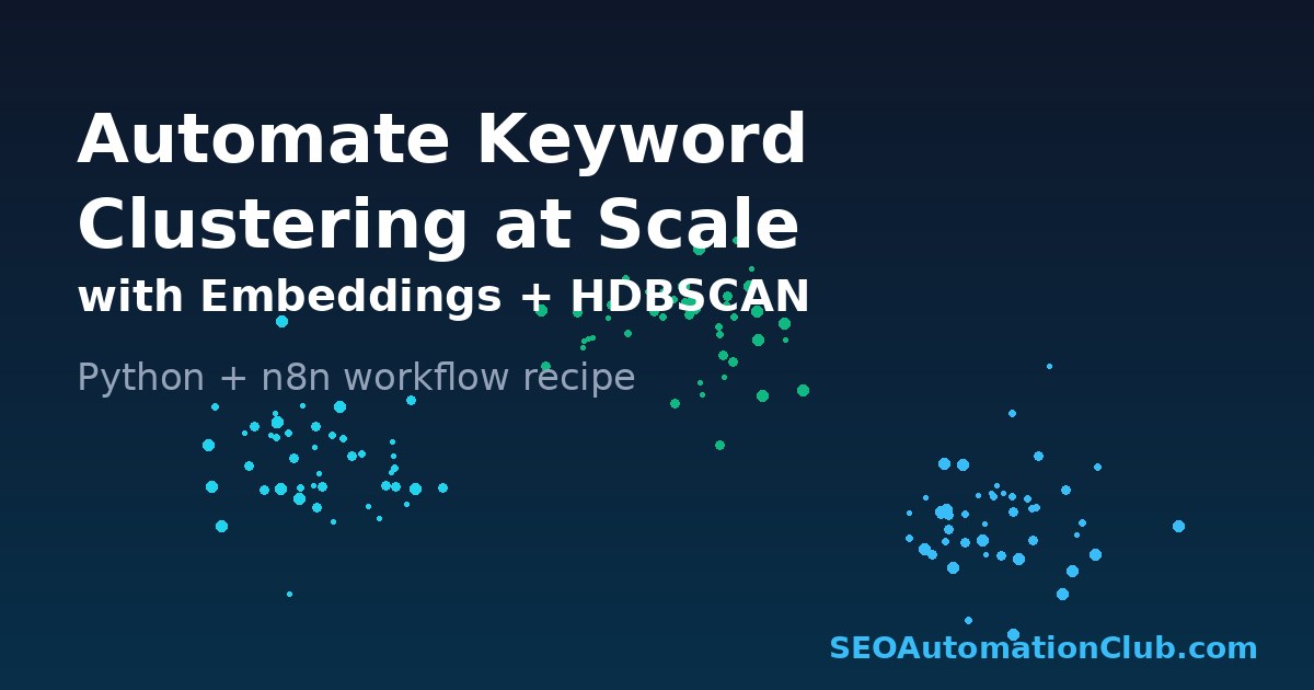
Automate Keyword Clustering at Scale: From a Raw Export to Content Topics with Embeddings + HDBSCAN
Keyword research tools hand you spreadsheets with 8,000 rows and zero structure. Somewhere in that list are 120 distinct articles waiting to be written — but figuring out which keywords belong to the same page is the part nobody automates well. Most teams either eyeball it (slow, inconsistent) or lean on the “group by lexical similarity” button inside a SaaS tool, which splits “how to fix crawl budget” and “crawl budget optimization” into two clusters because the words don’t overlap enough.
Lexical matching is the wrong tool. Search intent lives in meaning, not in shared tokens. This post walks through a clustering pipeline that groups keywords by semantic similarity using embeddings and density-based clustering — the same approach we use to turn a raw export into a ranked content backlog in a single n8n run. You’ll get the working Python, the parameter choices that actually matter, and the failure modes that quietly wreck your clusters.
Why embeddings beat lexical clustering for keyword grouping
A keyword’s value to SEO is its intent: the job the searcher wants done. Two queries can share no words and serve identical intent (“google not indexing my pages” vs “url inspection shows discovered currently not indexed”), while two queries can share most words and serve different intent (“best running shoes” vs “best running shoes for flat feet”). Token-overlap methods — TF-IDF, Levenshtein, n-gram Jaccard — only see the surface.
Embeddings encode each keyword as a vector positioned by meaning, so semantically related queries land near each other regardless of wording. Cluster those vectors and you get groups that map cleanly to “one page should target all of these.” We compared embedding providers for exactly this kind of SEO work in our embedding models teardown; for keyword clustering at the scale of a few thousand to a few hundred thousand terms, a small, cheap model like OpenAI text-embedding-3-small or open-source BGE is more than enough — clustering is forgiving of marginal embedding quality in a way that, say, reranking is not.
The pipeline, end to end
The flow has five stages: ingest the keyword export, embed each term, reduce dimensionality, cluster with HDBSCAN, then label and rank the clusters by opportunity. The first four are deterministic Python; the last benefits from an LLM. Here’s the core.
Step 1 — Embed the keywords in batches
import openai, numpy as np, pandas as pd

client = openai.OpenAI()
df = pd.read_csv("keywords.csv")  # columns: keyword, volume, difficulty
keywords = df["keyword"].str.strip().str.lower().tolist()

def embed(texts, model="text-embedding-3-small", batch=256):
    out = []
    for i in range(0, len(texts), batch):
        resp = client.embeddings.create(model=model, input=texts[i:i+batch])
        out.extend([d.embedding for d in resp.data])
    return np.array(out, dtype=np.float32)

vectors = embed(keywords)
Lowercasing and trimming before embedding matters more than it looks: it stops “Crawl Budget” and “crawl budget” from drifting apart and keeps duplicate detection trivial later. Batching at 256 keeps you well under token limits and cuts API round-trips by two orders of magnitude versus per-keyword calls.
Step 2 — Reduce dimensions before clustering
Embeddings are 1,536-dimensional. Density-based clustering degrades in high dimensions because distances become uniform — the “curse of dimensionality.” Reduce to 5–15 dimensions with UMAP first. This is the single highest-leverage step and the one most tutorials skip.
import umap

reducer = umap.UMAP(
    n_neighbors=15,      # higher = more global structure
    n_components=10,     # 5-15 is the sweet spot for clustering
    metric="cosine",     # embeddings are direction, not magnitude
    random_state=42,
)
embedding_2d = reducer.fit_transform(vectors)
Step 3 — Cluster with HDBSCAN, not K-Means
K-Means forces you to pick the number of clusters up front — absurd when you don’t know how many topics live in the list — and assigns every keyword to a cluster, including junk. HDBSCAN discovers the cluster count from the data and, critically, labels low-density points as noise (-1) instead of jamming them into the nearest group. Those noise points are usually your long-tail one-offs, and you want them flagged, not buried.
import hdbscan

clusterer = hdbscan.HDBSCAN(
    min_cluster_size=3,        # smallest group worth a page
    min_samples=1,             # lower = fewer points dumped as noise
    metric="euclidean",        # UMAP output, so euclidean is fine
    cluster_selection_method="leaf",  # tighter, more granular clusters
)
df["cluster"] = clusterer.fit_predict(embedding_2d)
The parameter that changes your output most is min_cluster_size. Set it to the smallest keyword group you’d build a page around — 3 is a sensible floor for content planning. cluster_selection_method="leaf" produces tighter, more specific clusters (better for article-level targeting); the default "eom" gives broader, hub-level groups. Run both and keep the one that matches your content model.
Step 4 — Label and rank clusters by opportunity
Now you have numbered clusters but no names. Pick the highest-volume keyword in each cluster as a cheap pivot, then have an LLM propose a working title and primary keyword. Rank clusters by total search volume divided by median difficulty so the backlog surfaces high-reward, low-effort topics first.
summary = (df[df.cluster != -1]
    .groupby("cluster")
    .agg(terms=("keyword", list),
         total_volume=("volume", "sum"),
         median_difficulty=("difficulty", "median"))
    .reset_index())
summary["opportunity"] = summary.total_volume / summary.median_difficulty.clip(lower=1)
summary = summary.sort_values("opportunity", ascending=False)
Feed each cluster’s term list to your model with a tight prompt — “Given these search queries, return a single article title and the primary keyword that covers them all” — and you have a prioritized content brief queue. From here it’s a short hop to our automated content brief pipeline, which takes each cluster and builds the full SERP-informed brief.
Wiring it into n8n for a repeatable run
Running this once in a notebook is fine for a one-off audit. To make it a habit — re-clustering every time you pull fresh keyword data — wrap it in n8n. A Schedule trigger kicks off a Code node (or an Execute Command node calling the Python script), the output writes to a Google Sheet or your CMS as draft briefs, and a final node posts the ranked cluster summary to Slack. Because HDBSCAN flags noise, you can route the -1 keywords to a separate “long-tail / FAQ candidates” tab automatically instead of losing them.
Failure modes that quietly ruin clusters
Three issues account for nearly every bad clustering run we’ve debugged. First, skipping dimensionality reduction — feed raw 1,536-dim vectors to HDBSCAN and you’ll get one giant cluster plus noise, because everything looks equidistant. Always reduce first. Second, brand and modifier noise: keywords containing your brand name or generic modifiers (“2026”, “free”, “best”) pull unrelated terms together. Strip or down-weight them before embedding. Third, treating noise as failure — a healthy run can legitimately mark 10–30% of a long-tail-heavy list as noise. That’s the algorithm protecting your clusters, not breaking them.
One more, related to overlap: clusters that look near-identical usually mean two pages competing for the same intent. That’s the same signal we chase in our content cannibalization detector — if two clusters sit on top of each other in vector space, you probably want one page, not two.
Results and takeaways
On a representative 8,400-keyword export, this pipeline collapsed the list into 214 content clusters in under four minutes of compute, with roughly 18% of terms flagged as long-tail noise for separate handling. The manual equivalent — a strategist grouping in a spreadsheet — typically runs a full day and produces inconsistent boundaries no two people agree on. The win isn’t only speed; it’s that the grouping is reproducible and defensible, driven by intent rather than someone’s Friday-afternoon judgment.
The bigger takeaway: keyword clustering is a solved problem once you stop matching strings and start matching meaning. Embeddings plus HDBSCAN plus a dimensionality-reduction step you can’t skip — that’s the whole recipe. Bookmark this if you run keyword research regularly; we publish a new automation playbook like this every week, and the clustering output feeds directly into the rest of the content pipeline.
Frequently asked questions
How many keywords can this handle?
UMAP and HDBSCAN scale comfortably to a few hundred thousand keywords on a single machine. The practical ceiling is usually your embedding API budget, not the clustering — and with text-embedding-3-small at fractions of a cent per thousand tokens, even a 200k-keyword run costs a few dollars.
Should I use K-Means instead of HDBSCAN?
Only if you specifically need a fixed number of clusters and have no long-tail noise — rare in real keyword data. HDBSCAN’s ability to discover the cluster count and isolate noise makes it the better default for content planning, where you don’t know how many topics exist in advance.
Do I need a paid embedding model?
No. Open-source BGE models run locally and cluster keywords nearly as well as paid APIs for this task, since clustering tolerates small embedding-quality differences. Paid models mainly save you the infrastructure of self-hosting. See our embedding model comparison for the trade-offs.
How often should I re-run the clustering?
Re-cluster whenever you pull a fresh keyword export — typically monthly, or after a major research push. Wiring it into n8n on a schedule means new keywords automatically fold into the existing topic map without manual work.
Trusted resources & further reading
For deeper, primary-source detail on the techniques referenced above, see:
Daniel Reyes — Operator & Editor, SEO Donna. Daniel Reyes is the operator behind SEO Donna. He oversees the automation engine that researches and drafts each article, and personally reviews every piece for accuracy and usefulness before it’s published. He works with small-business owners who want SEO handled for them.
Researched and drafted with SEO Donna’s automation engine, then reviewed by a human operator before publishing.